

The Dangerous Comfort of Executive Averages
Process capability analysis often begins with a number that appears reassuring: the average cycle time, average defect rate, average response time, or average output per shift. An arithmetic mean is easy to calculate and easy to place on an executive dashboard. It is also capable of concealing the operational conditions that create customer complaints, rework, overtime, and missed service commitments.
A process can report a stable mean while its defect tail expands, its best and worst performers separate, or two distinct operating patterns develop beneath the headline figure. By the time the average moves, the damage may already be visible in customer friction and escalating containment costs. Before funding a process redesign, leaders need to understand the distribution behind the mean, including variance, skew, outliers, clustering, and the stability of the measurement system.
How the Mean Disguises Root Operational Friction
An average compresses multiple dimensions of process behavior into one value. That compression is useful for high-level reporting, but dangerous when the number is treated as a complete description of performance. Two teams can produce the same mean cycle time while having entirely different levels of predictability. One may deliver nearly every transaction within a narrow range. The other may alternate between very fast and very slow work, producing the same average through mathematical cancellation.
That cancellation does not occur in the customer experience. A transaction completed ten minutes early does not necessarily compensate for another that arrives ten minutes late. In a regulated workflow, a single extreme delay may trigger a missed appointment, additional handling, or a compliance escalation. Similarly, one exceptionally low measurement can offset a high value in the average even though both observations indicate different process conditions.
Consider a healthcare workflow in which patient preparation, treatment administration, safety checks, room clearance, and contamination testing must occur in sequence. A published Lean Six Sigma project on outpatient iodine-131 therapy documented lengthy waits, inconsistent intervals between steps, and material waste as patient volume increased. The average process time could summarize the workload, but it would not identify whether delays originated in preparation, clinical verification, radiation surveys, or room release. The operational response requires empirical measurement of each stage, not confidence in a single aggregate. This is why clinical quality research on workflow variation is relevant even outside healthcare: systematic variation must be observed at the point where it occurs.
- Outliers may signal special causes, equipment failures, or exceptional handling requirements.
- Measurement noise can make a process appear more variable or more stable than it truly is.
- Skew can place a long tail of late or defective outcomes beyond what the mean suggests.
- Mixed populations can create a central average that represents no actual operating condition.
Why Capability Indices Collapse When Distributions Shift
Capability indices translate process behavior into a comparison with specification limits. Cp measures the width of the specification window relative to process spread, commonly expressed as six standard deviations. In simplified form, Cp equals the specification width divided by six times the standard deviation. It answers a limited question: can the observed spread fit within the allowed range if the process is centered?
Cpk adds the missing centering question. It compares the distance from the process mean to each specification limit, using the smaller distance. A process can therefore have a respectable Cp while producing a weak Cpk if its mean is too close to one limit. This distinction matters because customers and regulators experience the position of individual observations, not the theoretical width of a perfectly centered distribution.
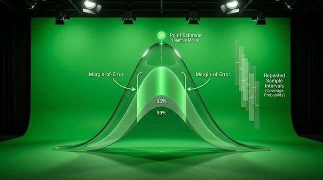
Distribution shifts make the difference even more consequential. Suppose a process has lower and upper specifications of 90 and 110, a mean of 100, and a standard deviation of 2. Under a normal approximation, Cp is about 1.67 and Cpk is also about 1.67. If the standard deviation rises to 3 while the mean remains 100, Cp falls to about 1.11, and the process has far less protection against defects. If the mean then shifts to 104, Cp remains about 1.11, but Cpk falls to about 0.67 because the upper limit is now much closer.
| Process condition | Mean | Standard deviation | Approximate Cp | Approximate Cpk | Operational meaning |
|---|---|---|---|---|---|
| Centered and tight | 100 | 2 | 1.67 | 1.67 | Strong protection on both sides |
| Centered but wider | 100 | 3 | 1.11 | 1.11 | More observations approach specifications |
| Wider and shifted | 104 | 3 | 1.11 | 0.67 | Upper-limit defects become likely |
| Mixed populations | 100 overall | Misleading aggregate | Not reliably interpretable | Not reliably interpretable | Subgroups must be analyzed separately |
These calculations also expose a limitation: Cp and Cpk are not automatically trustworthy for skewed or multimodal data. Standard deviation summarizes dispersion around the mean, but it does not explain whether observations form one stable population. A bimodal distribution may have a moderate overall standard deviation while containing two clusters, each generated by a different machine setting, operator method, shift, or material lot. The resulting capability index can describe neither subgroup accurately.
Diagnosing Bimodal and Skewed Patterns in Your Workflow
Unimodal assumptions fail when the process combines different operating conditions. A day shift and night shift may follow slightly different standard work. Two machines may share a nominal setting but respond differently under load. A batch process may alternate between material lots with different characteristics. When these populations are combined, a histogram can develop two peaks, a broad plateau, or a long tail. The overall mean may fall in the valley between clusters, where few actual observations occur.
Visual diagnosis should begin with a histogram, but it should not end there. Run charts reveal whether the observations change over time, while stratified plots show whether the pattern belongs to a particular operator, asset, product family, or shift. A stable-looking overall chart can conceal alternating behavior if data from separate streams are pooled. If a suspected bimodal pattern appears, analysts can use formal tools such as mixture models, distribution-fitting tests, the bimodality coefficient, or Hartigan”s dip test. The purpose is not to force a sophisticated model onto ordinary data. It is to determine whether one baseline is statistically defensible.
Precision measurement research provides a useful reminder that baseline diagnostics require verification of both the signal and the measurement system. A source such as advanced microsystems measurement research illustrates why highly precise engineering work depends on validated measurement behavior, even though the available article access does not establish specific findings for operational capability analysis. A Checking your browser prompt may appear before access to some research pages, but that access barrier is separate from the quality of the evidence. In practical terms, confirm calibration, repeatability, reproducibility, timestamp accuracy, and data lineage before interpreting small shifts as process changes.
- Use histograms to inspect shape, tails, gaps, and multiple peaks.
- Use run charts to identify trends, cycles, shifts, and sequences over time.
- Use box plots or percentile comparisons to expose subgroup differences.
- Check whether extreme observations are data errors, special causes, or genuine customer-impacting events.
- Do not delete outliers merely because they weaken the capability result.
A Five-Step Method to Rebuild Your Statistical Baseline
Rebuilding a baseline does not require abandoning executive metrics. It requires placing the mean in its proper role as one descriptive statistic among several. The baseline should explain how the process behaves, under which conditions, and with what level of confidence. A disciplined sequence also prevents teams from calculating capability indices before confirming that the underlying data is suitable.
- Test raw data for normality and multimodal clustering. Start with unaggregated observations and inspect histograms, probability plots, run charts, and summary percentiles. Use formal tests where appropriate, but interpret them alongside process knowledge. Large samples can flag trivial departures from normality, while small samples can miss meaningful structure.
- Stratify by shifts, machines, operators, and material lots. Recalculate center and spread within meaningful subgroups. If one machine or shift produces the long tail, the improvement target becomes specific rather than general. Maintain the original pooled view for business reporting, but do not use it as the only diagnostic baseline.
- Calculate Cp and Cpk alongside standard deviation and interquartile range. Cp and Cpk show specification performance under their assumptions. Standard deviation supports spread analysis, while the interquartile range provides a more robust view of the middle 50 percent when extreme values or skew distort the mean. Add percentiles such as P90, P95, or P99 when service delays and tail risk matter.
- Establish statistical control limits before long-term capability baselines. Control limits describe the expected behavior of a stable process; specification limits describe what customers or regulators require. Mixing these concepts creates confusion. First investigate special causes and stabilize the process, then calculate short-term and long-term capability using clearly defined windows.
- Build dashboards that highlight tail movement. Retain the mean, but pair it with median, standard deviation, percentile outcomes, defect rate, control signals, and subgroup comparisons. Alerts should trigger when the P95 cycle time rises, a cluster separates, or the distance to a specification limit narrows, even if the average remains unchanged.
Implementation also requires measurement-system discipline. If cycle times are recorded differently across teams, or defects are classified inconsistently, improved analytics will simply produce more precise confusion. Define the operational unit, start and stop points, inclusion rules, timestamp source, and treatment of rework before comparing periods. A baseline is credible only when the data-generation process is stable enough to support the conclusions drawn from it.
In a DMAIC program, this work belongs primarily in Measure and Analyze, but the benefit extends into Improve and Control. Once the hidden source of variation is isolated, countermeasures can target standard work, equipment settings, staffing patterns, material controls, or handoffs. Control plans should then monitor the variables that caused the original instability, rather than relying on a dashboard that reports only aggregate output.
Transform Your Operational Metrics into Reliable Growth Drivers
Operational leaders do not need to eliminate averages. They need to stop treating averages as evidence of stability. A mean is a useful centerline, but it cannot reveal distribution shape, subgroup behavior, tail exposure, or whether the process has shifted toward a specification boundary. Distributional integrity is the foundation for credible capability analysis and responsible capital allocation.
When teams validate the data, separate meaningful populations, monitor variation, and distinguish control limits from specifications, improvement decisions become more precise. Customer trust benefits because fewer extreme outcomes escape detection. Process investments produce stronger returns because resources are directed at the causes of variation rather than at symptoms hidden behind a compliant average. The discipline required today to rebuild a reliable baseline is substantially less costly than the engineering remediation, rework, and reputation damage created by an unstable process that looked healthy on a dashboard.